Sigproc

[[introduction]] Introduction ~~~~~~~~~~~~ These notes began life as a reply to a guy on the http://www.linux.ie/pipermail/ilug/[ILUG mailing list] regarding how to get some information on the frequency content of noise from electrical transformers using tools on a Linux system. I felt I had a useful approach, so I put it together in an email, and here I present some of the points. This is, of course, not an in-depth look at the topic, or authoritative, but it is a quick overview and perhaps a useful tutorial to students or others taking a first cut at this problem. The tools/programs you will need are: * http://www.alsa-project.org/[ALSA] * http://sox.sourceforge.net/[sox] * http://www.python.org/[Python], including the https://pypi.org/project/Numeric/#Numeric[Python Numeric] extensions. * http://www.gnuplot.info[Gnuplot] All of this software is freely available, and it is quite likely that most of it is included on your GNU/Linux distribution's installation media. [[instructions]] Instructions ~~~~~~~~~~~~ [[recording-a-sound-sample]] Recording a Sound Sample ^^^^^^^^^^^^^^^^^^^^^^^^ I only use the http://www.alsa-project.org/[ALSA] sound architecture for GNU/Linux, and I find it very good. I have some notes on link:alsa_help.html[how to install] ALSA which might be helpful, though they are probably a little out of date by now. Recording uses the _arecord_ program, which is in the alsa-utils. There is a high chance it is already installed on your system if you installed ALSA from your distribution. You use alsamixer to set the channel you want to record from. This will probably be the microphone channel (space-bar switches capture on). You also need to activate microphone boost. On my setup, with a soundblaster, i do this by unmuting (M toggles the mute setting). You could also acquire your sound sample from a CD, or from line in. It's up to you. An example invocation of arecord would be:

arecord -d 5 -f S16_LE -c1 -r44100 out.wav

This will record 5 seconds, 1 channel (mono), with a sampling rate of 44.1kHz (the same as CD audio). The output is a wav file, with 16 bits per sample (two bytes), and Linear Encoding. There are other options you can use, but these are a good place to start. In particular, i think it is best to work in mono unless you have good reasons to do otherwise (I don't, and I have not investigated the complications). It is probably a good idea to listen to the sample you have just recorded, to check it is what you think it is. You can do this using

aplay out.wav

or by playing the wav in http://www.xmms.org/[xmms] or whatever you like. [[converting-the-sound-sample]] Converting the Sound Sample ^^^^^^^^^^^^^^^^^^^^^^^^^^^ To process the sound sample, I needed to have the samples in essentially an ASCII text-file format. There are various ways to do this, and I have used several as a consequence of initially being ignorant of the "Right Way To Do Things". In truth, i probably still do not know the "Right" way, but I'll describe a few of your options. Sox is a fantastic utility for converting sound file formats. One option it has is to convert to the "dat" file format. It is described like this in the man page: .... .dat Text Data files These files contain a textual representation of the sample data. There is one line at the beginning that contains the sample rate. Subsequent lines contain two numeric data items: the time since the beginning of the first sample and the sample value. Values are normalized so that the maximum and minimum are 1.00 and -1.00. This file format can be used to create data files for external programs such as FFT analyz ers or graph routines. SoX can also convert a file in this format back into one of the other file formats. .... Using sox in this way is simplicity itself:

sox out.wav out.dat

The first line in out.dat starts with a ";", and has info on the sample rate. The dat file produced here is very easy to read into a python program (or indeed a program in any language). It is also suitable for immediate plotting with http://www.gnuplot.info[Gnuplot] if you strip off the initial line containing the semicolon (or put a "#" at the start). Before I realised that sox had done all my work for me I tried a couple of other options. These aren't clever or smart, but they show how easy it can be to mess around with sound formats. The first thing I tried was a solution completely implemented in python. This was slow, but it did work. The code went as follows:

import wave audioop
wav_in=wave.open('out.wav','r')
contents=w.readframes(w.getnframes())
# contents now holds all the samples in a long text string.
samples_list=[]; ctr=0
while 1:
    try:
        samples_list.append(audioop.getsample(contents,2,ctr))
        # "2" refers to no. of bytes/sample, ctr is sample no. to take.
        ctr+=1
    except:
        # We jump to here when we run out of samples
        break
o=open('outfile.dat','w')
for x in range(len(out)):
    o.write('%d %e\n'%(x,out[x]))

Another, only slightly different approach was to use sox first (remember, I didn't know what sox could do when i tried this!), to turn our wav file into a raw file, with signed samples, and two bytes (1 word) per sample:

sox out.wav out.sw

Then back to python, and do:

contents=open('m.sw','r').read()

At this point, "contents" has the same form as it did in the previous python code, and the output can proceed as before. As a final aside, it might be of interest to know that it is very easy to write a small C program to take the out.sw file above and turn it into a "dat" style file with one sample per line. The code is in convert.c. Ultimately it is useless, as it does nothing sox doesn't do, but it is very very quick compared to the python implementation (No surprise, I suppose, but I was still a little taken aback by the speed gain even with my limited C coding experience). [[analysing-the-signal]] Analysing the Signal ^^^^^^^^^^^^^^^^^^^^ This is really quite easy, assuming you have http://www.pfdubois.com/numpy/#Numeric[Numerical Python] and the FFT modules installed. Continuing from our last code snippet, where "out" contains a list of the samples from our sound file, the following gives us an FFT:

import Numeric
import FFT
out_array=Numeric.array(out)
out_fft=FFT.fft(out)

It is as easy as that! To put the FFT data in a file suitable for plotting in Gnuplot, the following code was used:

offt=open('outfile_fft.dat','w')
for x in range(len(out_fft)/2):
    offt.write('%f %f
'%(1.0*x/wtime,abs(out_fft[x].real)))

Now, depending on your knowledge of FFT's (Fast Fourier Transforms) the above might need some explanation. First of all, the FFT data produced will be complex. However, we are looking at a purely real signal, so we will discard the Imaginary part. Also, only half the data is useful, as the other half is just a mirror image (if you looked at the imaginary part, it would be a mirror image multiplied by -1). Also, you can look on the index of the FFT as meaning the number of cycles occurring in the time-duration of the total sound extract. Thus, the 0, first component is the DC component. The index 1 sample reverses once in the time duration, the next one reverses twice, and so on (lowest frequency is on the left!). [[viewing-the-results]] Viewing the Results ^^^^^^^^^^^^^^^^^^^ To view the output, you need to use some graphing software. http://www.gnuplot.info[Gnuplot] is one good option. Included below are thumbnails (links to full size) of an link:out.mp3[original time-domain signal], followed by the entire FFT data (as output to file by the python code above). And a smaller detail of the region where most of the interest is, between 1000 and 2000 Hz. 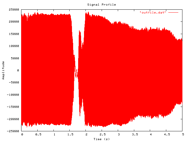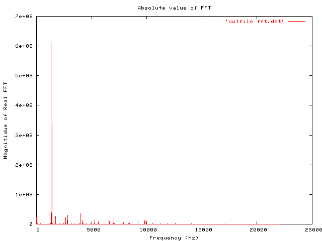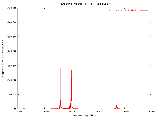.Time domain plot of input signal image:/timeplot.png["Time Plot", width=128, link="/timeplot.png"] .Plot of overall FFT data image:/fft_plot_a.png["Overall FFT data", width=128, link="/fft_plot_a.png"] .Detailed plot of FFT data, range 1-2kHz image:/fft_plot_b.png["Detailed FFT", width=128, link="/fft_plot_b.png"] Gnuplot code to produced these figures is included below:

set style data lines
# Time domain signal first:
set xlabel 'Time (s)'; set ylabel 'Amplitude'
set title 'Signal Profile'
set terminal png
set output 'timeplot.png'
plot 'outfile.dat'
# Now look at FFT Data
set output 'fft_plot_a.png'
set xlabel 'Frequency (Hz)'
set ylabel 'Magnitude of Real FFT'
set title 'Absolute value of FFT'
plot 'outfile_fft.dat'
# Now get a closer look at where the action is...
set xrange [1000:2000]
set title 'Absolute value of FFT (Detail)'
set output 'fft_plot_b.png'
replot

For what it's worth, the signal analysed here is a 5 second (220500 samples) recording of two notes from a harmonica. [[conclusion]] Conclusion ^^^^^^^^^^ These have just been some quick and sketchy notes on how to analyse a sound input and find out what frequency content it has. As you can see, there is nothing very clever or difficult to the implementation of this, but it is still (in my opinion!) interesting to do. If you have more interesting sound inputs to work on (e.g. vibrations from a machine) you could proceed even further with your analysis and use it as a tool for locating the source of the vibration and noise. There may be typos in the code snippets in this article. However, you can download the link:/sigproc.tar.gz[archive of code] [Not up yet], which I have run and used to produce the figures included above. Even though that does not mean there are no mistakes, it does at least mean you can reproduce my results (Note that the sound sample is included in mp3 format, to save my webspace and bandwidth, so you will have to first convert it to a wav file. http://www.xmms.org[xmms] can do this for you using its cdwriter plugin (plays an mp3 into a wav file)). [[future-work-links]] Future Work, Links ~~~~~~~~~~~~~~~~~~ An obvious further development would be to do a wavelet transform on the sound signal. Hopefully when I have a bit more spare time I'll put something on this topic up here. A useful link I http://www.linux.ie/pipermail/ilug/2002-October/051187.html[saw on ILUG] is http://www.cf.ac.uk/psych/CullingJ/pipewave.html[Pipewave] which is a suite of command line tools for stuff like this. AFAICS, the emphasis is on speech applications, but should be of general interest too. >> Home

2018/07/15